FactSage Modules – FactSage Software and Databases

View Data
Compound
Solution
Reaction
Predom
EpH
Equilib
Phase Diagram
Calphad Optimizer
Results
Mixture
Fact-XML
Figure
Viscosity

1. View Data

Click on Download View Data Show (pdf presentation – 36 pages) for detailed information on View Data.

View Data scans the databases and enables you to display the standard state thermodynamic properties of the compound species and to list the solution phases. (To edit, modify and save new data use Compound and Solution.)

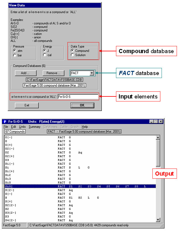
Fig. 1 – Listing all Fe-Si-O-S species stored in the FACT compound database

For example, Fig. 1 shows how to list all stoichiometric compounds involving the elements Fe-Si-O-S that are stored in the FACT compound database. The mouse has been clicked on SiO2 where it is noted that the compound has 8 solid allotropes (s1 to s8) and a liquid phase (L).

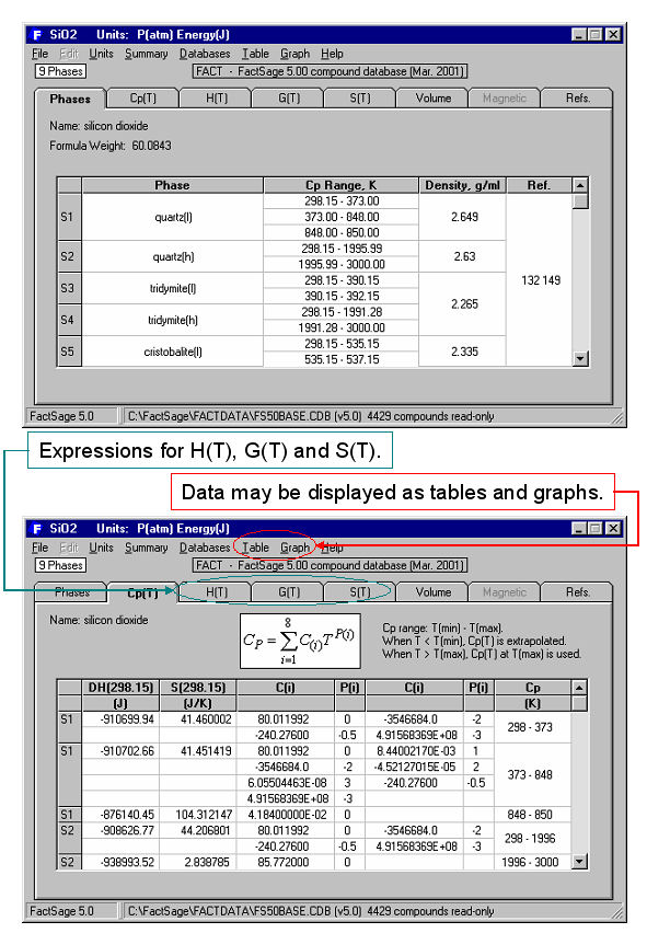
Fig. 2 – Summary of phases (top) and compound data (bottom) for SiO2.

By double clicking on SiO2 in Fig. 1, you generate the output in Fig. 2 which shows a summary of phases and a partial listing of the ΔHº(T), Sº(T) and Cp(T) compound data for SiO2.

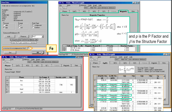
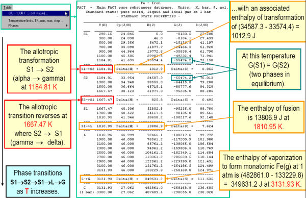
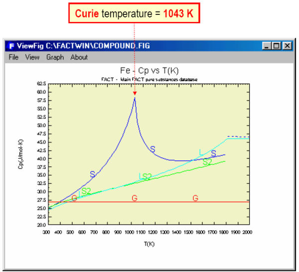
Fig. 3 shows the magnetic thermodynamic data as well as other thermodynamic data for Fe. In Fig. 4 the data for Fe are displayed in tabular format for the temperature range 298.15 to 3300 K – note the transition temperatures and associated changes (delta values) in the thermodynamic properties. The Cp values for Fe are plotted in Fig. 5.

Other data which are stored in the compound databases, and which can be accessed by the View Data include non-ideal gas constants, molar volumes, expansivities, compressibilities, and derivatives of the bulk moduli.

Fig. 3 – Magnetic data and Cp expression for Fe.

2. Compound

Click on Download Compound Slide Show (pdf presentation – 50 pages) for detailed information on Compound.

Compound is used to copy, enter, edit, list and store data in your private compound (pure substances) databases.

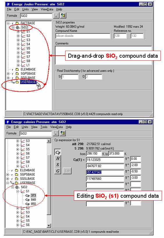
Fig. 1 – Top: drag-and-drop of SiO2 data from the FACT to the private USER database. Bottom: manipulation of Cp(T) data in the USER database.

For example, in Fig. 1 by using ‘drag and drop’, SiO2 is copied from the read-only (r) FACT database (FACTBASE) into a private read/write (r/w) database USERBASE where the Cp(T) expressions for quartz, SiO2(s1) are being modified.

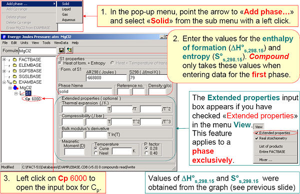
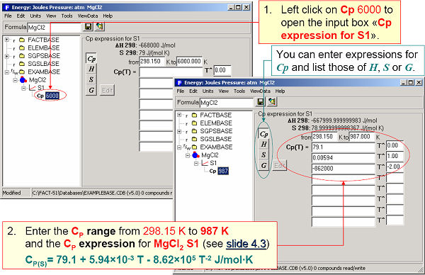
Fig. 2 – Add a compound to the database: H298 and S298 for 1st phase.

In Fig. 2 ΔH298K and S298K are entered for the solid phase of MgCl2. Cp(T) expressions are entered in Fig. 3.

Fig. 3 – Add a compound to the database Cp values for the 1st phase.

3. Solution

Click on Download Solution Slide Show (pdf presentation – 42 pages) for detailed information on Solution.

Solution is used to enter, edit, list and store non-ideal mixing properties in your private solution databases.

4. Reaction

Click on Download Reaction Slide Show (pdf presentation – 37 pages) for detailed information on Reaction.

Reaction is used to calculate changes in extensive thermodynamic properties (H, G, V, S, Cp, A) for a single species, a mixture of species or for a chemical reaction. The species may be pure elements, stoichiometric compounds or ions (both plasma and aqueous ions).

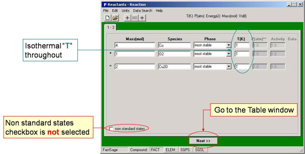
Fig. 1 – Cu-O2-Cu2O system. Entry of the isothermal standard state reaction for copper oxidation.

For example, Fig. 1 shows the entry of the isothermal standard state reaction for the oxidation of copper:

4 Cu + O2 = 2 Cu2O

Note that the phases are not specified (i.e. most stable is requested).

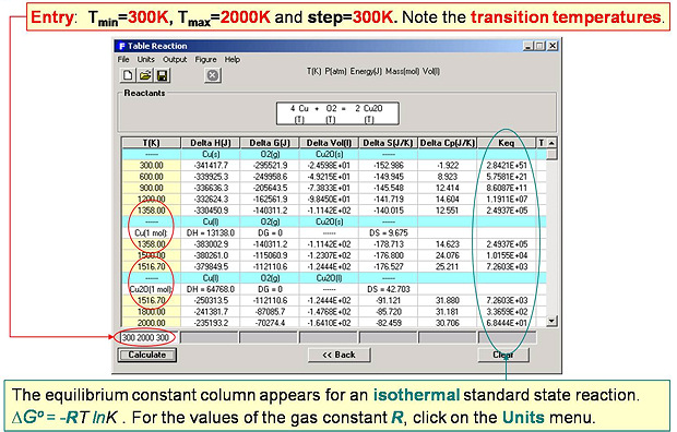
Fig. 2 – Cu-O2-Cu2O system. Calculation of common thermodynamic values.

In Fig. 2 the T(K) temperature range (300 to 2000 in steps of 300) is entered and Reaction determines the most stable phases at each temperature and lists common thermodynamic values including the transition temperatures.

For example at 1200 K the stable standard state phases are Cu(s), O2(g), Cu2O(s), and the changes in the standard state properties are ΔHº = -332.62 kJ, ΔGº = -162.43 kJ, ΔSº = -141.83 J/mol-K, Keq = 1.176 x 106. All the common thermodynamic equations are respected, for example:

ΔGº = ΔHº – T ΔSº = – R T ln Keq

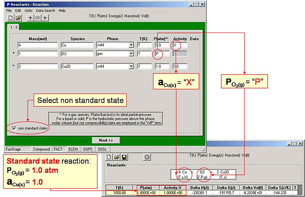
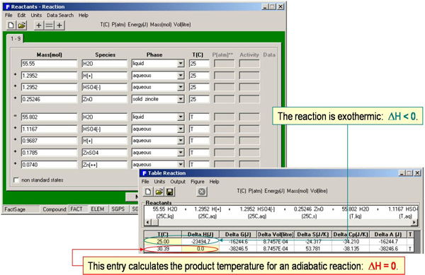
Fig. 3 – Cu-O2-Cu2O system. Entry of the isothermal non-standard state reaction for copper oxidation.

Fig. 3 shows entry of the non-standard state reaction:

4 Cu(s, activity X) + O2(g,Po2) = 2 Cu2O(s)

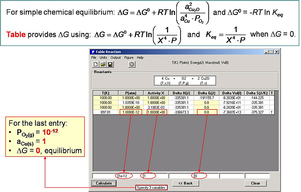
Fig. 4 – Cu-O2-Cu2O system. Calculation of thermodynamic values by the interactive spreadsheet format.

In Fig. 4 the power of the interactive spreadsheet output format of Reaction is demonstrated. For example, in line 1 the user sets the activity of Cu(s) and the partial pressure of O2 at standard conditions (a = X =1, P = 1) and the changes in the standard enthalpy (ΔHº = -33.54 kJ), Gibbs energy (ΔGº = -191.16 kJ) etc. are calculated at 1000 K. In line 2, with the activity of Cu(s) still set to unity (X = 1.0), the Gibbs energy change is set to zero (i.e. equilibrium) and the equilibrium oxygen pressure is calculated to be Po2 = 1.0359 x 10-10 atm. In line 3 the equilibrium activity of Cu(s) is calculated (3.1903×10-3) when Po2 = 1.0 atm. In the last entry (line 4) O2 with Po2 = 10-12 atm and Cu with a(Cu(s)) =1 are at equilibrium (ΔG = 0) at the calculated temperature 897.01 K.

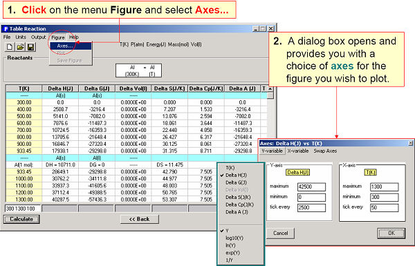
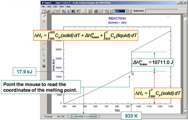
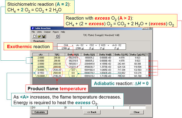
Reaction is a simple and effective teaching tool in giving students a ‘feel’ for thermochemical calculations. It is not limited to isothermal reactions and equilibrium constants. By appropriate entries you can perform heat balances, calculate adiabatic flame temperatures (by setting ΔH = 0), solve simple equilibria, determine vapor pressures, calculate aqueous solubilities, etc. The results may also be automatically displayed as graphs and stored or exported in the form of spreadsheets (for example Excel®).

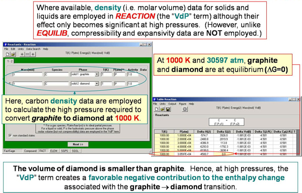
For example, the enthalpy requirements to heat Al(s) from 300 K to various temperatures are calculated in Fig. 5 and plotted in Fig. 6. Fig. 7 illustrates a variety of calculations for the simple combustion of methane in excess oxygen. Fig. 8 shows the effect of the ‘VdP’ term and high pressure on the graphite to diamond transition. Fig. 9 involves aqueous chemistry and demonstrates a thermal balance for the leaching of zinc oxide.

Fig. 5 – Heating Al: setting the graphical display with Figure.

Fig. 6 – Heating Al: a few thermodynamical considerations.

Fig. 7 – Combustion of methane in excess O2 – adiabatic reactions.

Fig. 8 – Effect of high pressure on the graphite to diamond transition.

Fig. 10 – Thermal balance for leaching of zinc oxide.

5. Predom

Click on Download Predom Slide Show (pdf presentation – 34 pages) for detailed information on Predom .

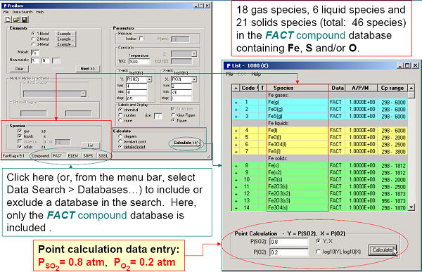
Predom enables you to calculate and plot isothermal predominance area diagrams for one-, two or three-metal systems using data retrieved from the compound databases.

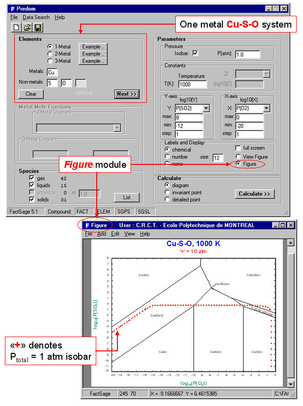
Fig. 1 – Top: entry of the one-metal Cu-p(SO2)-p(O2) system at 1000K. Bottom: resulting calculated predominance diagram.

For example, Fig. 1 shows the entry and resulting diagram for the one-metal Cu-Pso2-Po2 system at 1000 K. After the components (Cu, S and O) have been specified, the user is presented with a list of possible axes, log10X and log10Y (X and Y are pressure or activity of S, S2, …Sn, SO, SO2, SO3, O2 etc.), and possible product species (gases, solids, liquids – these may be edited by clicking on the “List” button). A useful feature of the program is the option to include the calculated total pressure isobar on the predominance diagram (plotted as “+”s in Fig. 1). Along such an isobar the total pressure is the sum of the partial pressures of all the gaseous species (in Fig. 2, P(total) = 1 atm = Ps + Ps2 + … Psn + Pso + Pso2 + Pso3 + Po2 + Pcu … etc.). Such a line represents the reaction path whereby, for example, Cu2S oxidizes to, say, Cu2O.

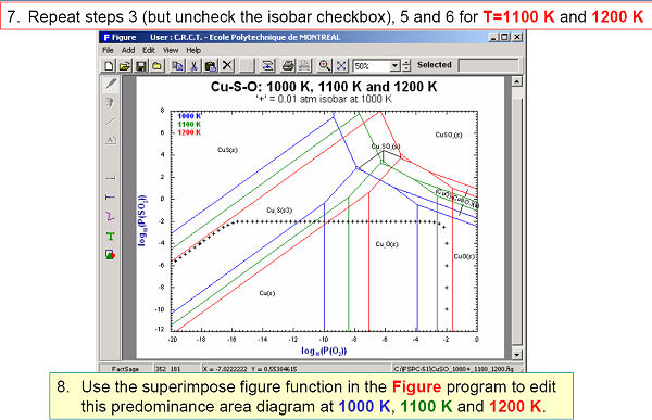
Fig.2 – Superimposed Predom diagrams for Cu-SO2(g)-O2(g) at 1000, 1100 and 1200K.

Fig 2. shows the effect of temperature on the Cu-Pso2-Po2 system.

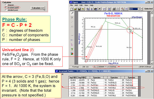
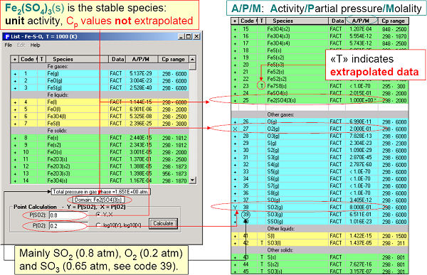
Fig. 3 – Invariant points of Fe-SO2(g)-O2(g) at 1000K.

Fig 3. displays the calculated diagram and invariant points of Fe-Pso2-Po2 at 1000 K. A detailed point calculation at Pso2 = 0.8 atm and Po2 = 0.2 atm is presented in Figs 4 and 5.

Fig. 4 – Detailed point calculation at Pso2 = 0.8 atm and Po2 = 0.2 atm for Fe-SO2(g)-O2(g) at 1000K.

Fig. 5 – Detailed point calculation at Pso2 = 0.8 atm and Po2 = 0.2 atm for Fe-SO2(g)-O2(g) at 1000K.

The calculated diagrams can be stored as figure (*.fig) files, edited by Figure, and exported as *.bmp, *.emf and *.wmf files.

Predom also enables you list the coordinates all the invariant points as well as perform detailed equilibrium calculations at any point on the diagram.

6. EpH

Click on Download EpH Slide Show (pdf presentation – 30 pages) for detailed information on EpH.

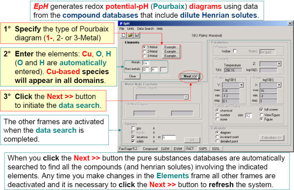
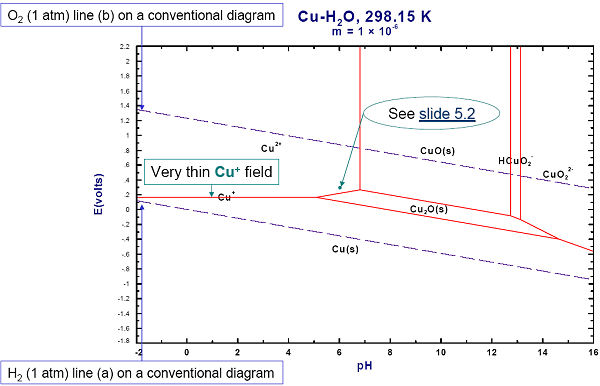
EpH enables you to generate isothermal Eh vs. pH (Pourbaix) diagrams for one-, two or three-metal systems using data retrieved from the compound databases that also include infinitely dilute aqueous data. Note: EpH only accesses compound databases – the aqueous phase is treated as an ideal solution.

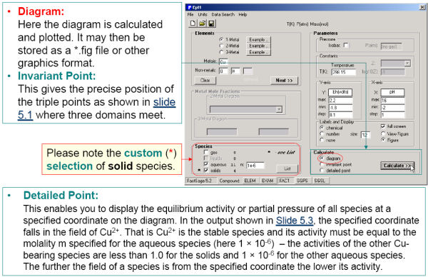
Figs. 1 to 3 show the input and resulting Eh-pH diagram for the Cu-water system.

Fig. 1 – The Cu-water Eh-pH diagram: the Elements frame.

Fig. 2 – Specifying the Cu water Eh-pH diagram: the Calculate frame.

Fig. 3 – Cu-H2O Eh-pH diagram: Graphical Output.

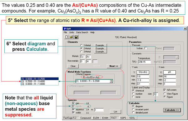
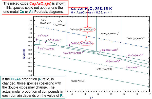
Figs. 4 and 5 show how to generate a ‘two-metal’ Eh-pH diagram for the Cu-As-water system. Since the stabilities of the Cu and As mixed compounds (Cu3(AsO4)2(s) and Cu3As(s)) depend upon the relative amounts of Cu and As, it is also necessary to define the range of the metal mole fraction R, As / (As + Cu).

Fig. 4 – The Cu-As-water Eh-pH diagram: the Metal Mole Fraction frame.

Fig. 5 – The Cu-As-water Eh-pH diagram: graphical output.

The calculated diagrams can be stored as figure (*.fig) files, edited by Figure, and exported as *.bmp, *.emf and *.wmf files.

EpH also enables you list the coordinates all the invariant points as well as perform detailed equilibrium calculations at any point on the diagram. You can also calculate diagrams under constant partial gas pressures.

7. Equilib

Click on Download Equilib Regular Slide Show (pdf presentation – 102 pages) for detailed information on the regular features of Equilib. Click on Download Equilib Advanced Slide Show (pdf presentation – 115 pages) for detailed information on the advanced features of Equilib .

Equilib is the Gibbs energy minimization workhorse of FactSage and the most popular program. It calculates the concentrations of chemical species when specified elements or compounds react or partially react to reach a state of chemical equilibrium. In most cases the user makes three entries as shown in the Equilib Reactants Window (Fig. 2) and Menu Window (Fig. 3):

1st entry: Define the reactants, then click on ‘Next >>’.
2nd entry: Select the possible compound and solution products.
3rd entry: Set the final conditions – T and P, or other constraints, then click on ‘Calculate >>’.

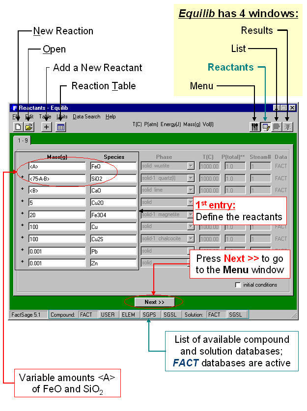
Fig. 1 – Reactant Window Cu-matte-slag system. Entry of the rectants including a variable amount of FeO and SiO2.

The Reactants Window (Fig. 1) shows the entry for a copper-based pyrometallugical system (variable amounts <A> of FeO, <75A – B> of SiO2, and <B> of CaO, with fixed amounts of Cu2O, Fe2O3, Pb, Zn, Cu and Cu2S).

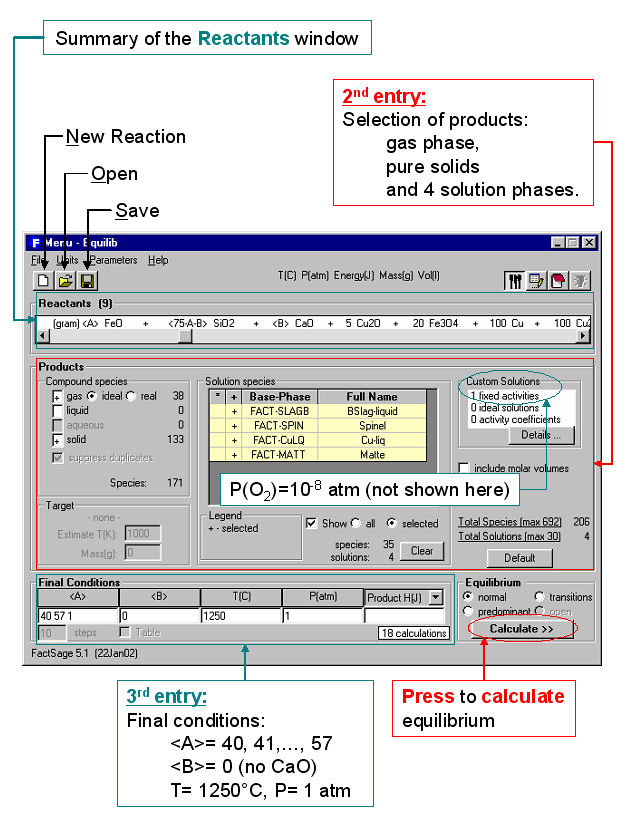
Fig. 3 – enu Window Cu-matte-slag system. Selection of possible product phases and definition of the final conditions

In the Menu Window (Fig. 3) the possible products are identified (gas phase, pure solids and slag, spinel, matte, copper alloy solution phases) together with a range of composition (<A> = 40, 41, 42, … 57), the temperature (1250ºC) and total pressure (1 atm.). Not shown here is how one can set various constraints, options, targets, etc. (in the example the equilibrium partial pressure of oxygen was fixed at P(O2) = 10-8 atm). You then click on the “Calculate >>” button and the computation commences.

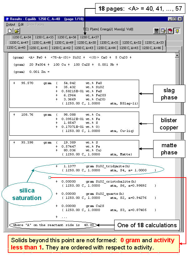
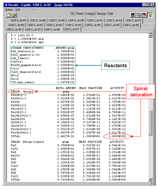
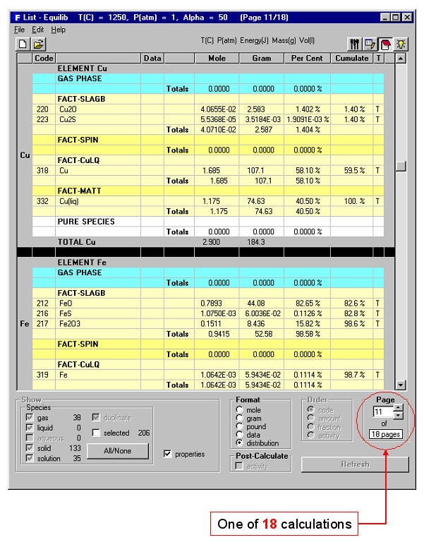
When the calculation is finished you are automatically presented with the Results Window where Equilib provides the equilibrium products of the reaction and where the results may be displayed in F*A*C*T and ChemSage output formats. The equilibrium product amounts are positive, satisfy the mass balance constraints with respect to the system components and correspond to the lowest possible Gibbs energy for this particular selection of possible products. For example Fig. 3 displays the results in F*A*C*T format at <A> = 40; this equilibrium point corresponds to silica saturation, a(SiO2) = 1.0. The equilibrium compositions of the slag, matte and blister copper are also listed. Fig. 4 shows a ChemSage output format for <A> = 57 that now corresponds to spinel saturation. The calculated values may also be presented and manipulated via the List Window. For example Fig. 5 shows the distribution of the elements (Cu, Fe) among the phases when <A> = 50.

Fig. 3 – Results Window Cu-matte-slag system. Display of the results in F*A*C*T Format for silica saturation (=40).

Fig. 4 – Results Window Cu-matte-slag system. Display of the results in ChemSage Format for spinel saturation (=57).

Fig. 5 – List Window Cu-matte-slag system. Distribution of the elements (Cu, Fe) among the phases when =50.

You may enter up to 48 reactants consisting of up to 32 different components (elements and electron phases). Reactants may include “streams” – these are equilibrated phases stored from the results of previous calculations (useful in process simulation). Phases from the compound and solution databases are retrieved and offered as possible products in the Menu Window. These may include pure substances (liquid, solid), ideal solutions (gas, liquid, solid, aqueous) and non-ideal solutions (real gases, slags, molten salts, mattes, ceramics, alloys, dilute solutions, aqueous solutions, etc.) from the databases described earlier.

Equilib employs the Gibbs energy minimization algorithm and thermochemical functions of ChemSage and offers great flexibility in the way the calculations may be performed. For example, the following are permitted: a choice of units (K, C, F, bar, atm, psi, J, cal, BTU, kwh, mol, wt.%, …); dormant phases in equilibria; equilibria constrained with respect to T, P, V, H, S, G, U or A or changes thereof; user-specified product activities (the reactant amounts are then computed); user-specified compound and solution data; and much more. Phase targeting and one-dimensional phase mappings with automatic search for phase transitions are possible. For example, you can calculate all equilibrium (or Scheil-Gulliver non-equilibrium) phase transitions as a multicomponent mixture is cooled.

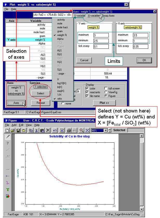
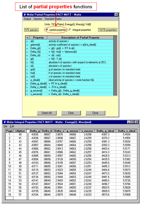
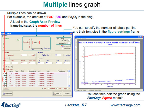
Equilib offers a post-processor whereby the results may be manipulated in a variety of ways: tabular output ordered with respect to amount, activity, fraction or elemental distribution; post-calculated activities; user-specified spreadsheets of f(y) where y = T, P, V, H, S, G, U , A, Cp or species mole, gram, activity, mass fraction and f = y, log(y), ln(y), exp(y) etc. for Lotus 1-2-3, Microsoft Word or Excel. For example Fig. 6 shows post-processing of the results and the generation of a Cu wt%. vs Fe(total)/SiO2 wt.% diagram for the complete set (18) of equilibrium calculations. Fig. 7 shows (top) a display of the thermodynamic partial properties functions, and (bottom) a partial listing of the calculated integral properties of a solution phase (FACT-MATT) for all 18 calculations.

Fig. 6 – Post-processor Window Cu-matte-slag system. Defining and plotting a Cu wt.% vs Fe(total)/SiO2 wt.% diagram for all results (=40 to 57).

Fig. 7 – Solution Properties Window Cu-matte-slag system. Top: list of the partial properties functions. Bottom: calculated integral properties of the matte phase.

8. Phase Diagram

Click on Download Phase Diagram Slide Show (pdf presentation – 162 pages) for detailed information on the Phase Diagram Module.

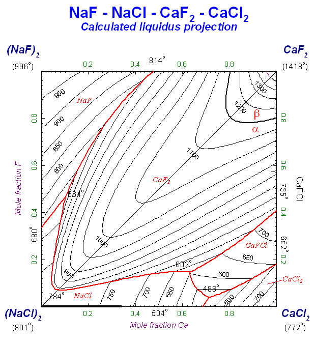
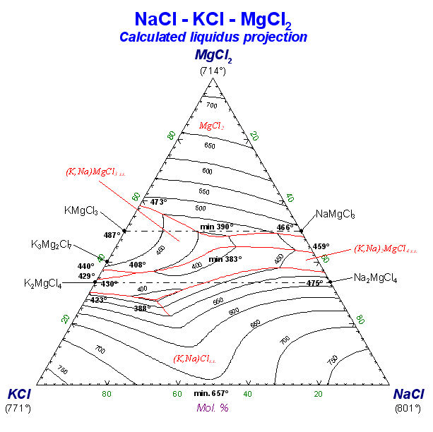
Phase Diagram is a generalized module that permits one to calculate, plot and edit unary, binary, ternary and multicomponent phase diagram sections where the axes can be various combinations of T, P, V, composition, activity, chemical potential, etc. The resulting phase diagram is automatically plotted by the Figure module. It is possible to calculate and plot: classical unary temperature versus pressure, binary temperature versus composition, and ternary isothermal isobaric Gibbs triangle phase diagrams; two-dimensional sections of a multi-component system where the axes are various combinations of T, P, composition, activity, chemical potential, etc.; predominance area diagrams (for example Pso2 vs Po2) of a multicomponent system (e.g. Cu-Fe-Ni-S-O) where the phases are real solutions such as mattes, slags and alloys; reciprocal salt phase diagrams; etc.

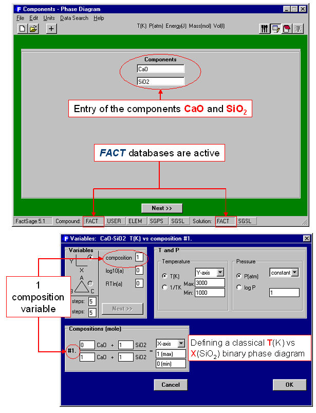
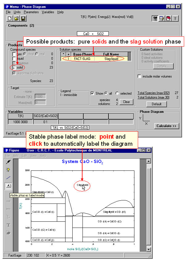
Fig. 1 – CaO-SiO₂ system. Top: Components Window – entry of CaO and SiO2. Bottom: Variables Window – selection of T(K) and X(SiO2) axes.

Fig. 2 – CaO-SiO₂ system. Top: Menu Window – selection of the possible products. Bottom: Figure Window – resulting binary CaO-SiO2 phase diagram.

The calculation of the binary temperature versus composition phase diagram for the CaO-SiO2 system is shown in Figs. 2 and 3 In the Phase Diagram module the system components (CaO, SiO2) are first entered in the Reactants Window (Fig. 1 top). Then the type of phase diagram is defined in the Variables Window (Fig. 1 bottom) where the user selects the type of diagram (Y vs X, or Gibbs triangle), the type of axes (composition, activity and chemical potential), the possible composition variables, and the limits and constants of the phase diagram. Data from the compound and solution databases are offered as possible product phases in the Menu Window (Fig. 2 top). In the case of CaO-SiO2, the slag solution phase (FACT-SLAG) and all pure solids (including those outside the plane CaO-SiO2) are selected as possible product phases. By clicking on the ‘Calculate >>’ button the phase diagram is automatically calculated and plotted in real time (Fig. 2 bottom). When the calculation is complete the Figure module uses the graph as a dynamic interface. By pointing to any domain, tie lines and stable phases are automatically labeled. Optionally the figure can be manipulated: tie lines can be inserted in the plot, the equilibrium compositions and phase amounts at any point on the diagram can be calculated and shown in a table, and the diagram can be edited (add experimental data points, text, change font and colors etc.). Examples of edited diagrams are shown later.

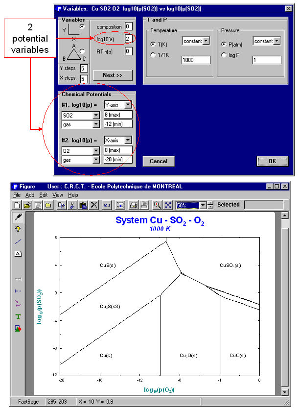
Fig. 3 – Cu-SO₂-O₂ system. Top: selection of the log1010(Pso2) and log10(Po2) axes at 1000K. Bottom: the resulting predominance area diagram.

The versatility of the choice of axes in the Variables Window enables one to generate many different types of phase diagrams. Fig. 3 is a classical isothermal predominance area diagram for the Cu-SO2-O2 system. The system components are Cu, SO2, O2; the axis variables are log10(Pso2) and log¨10(Po2) and the temperature is set constant; the possible phases in the phase diagram are gas and stoichiometric solids taken from the FACT compound database. This diagram may be compared to the one produced by the Predom module for the same system.

Fig. 4 – Fe-Cr-O₂ system. Top: selection of FACT(oxide) and SGTE(alloy) solution phases. Bottom: resulting log10(Po2) vs Cr/(Cr+Fe) phase diagram at 1573K.

Fig. 5 – FeO-TiO2-Fe System. Top: selection of the axes at constant Fe content. Bottom: resulting T(C) vs TiO2/(FeO+TiO2) isopleth at 50 mol% Fe.

Fig. 6 – FeO-TiO2-Fe system. Example of the phase equilibrium mode calculation at the coordinates 1450ºC and TiO/(FeO+TiO2) = 0.7.

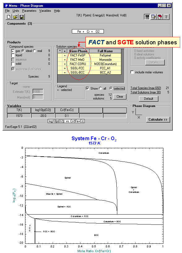
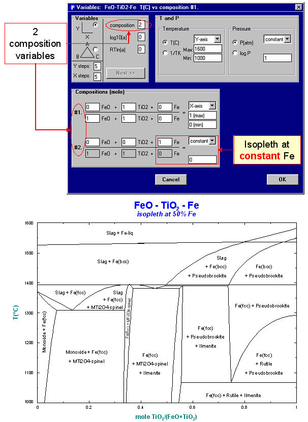
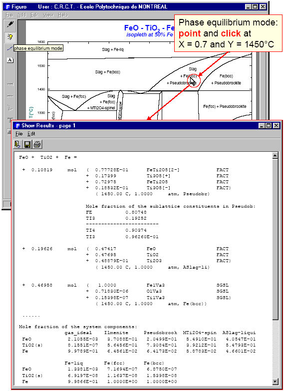
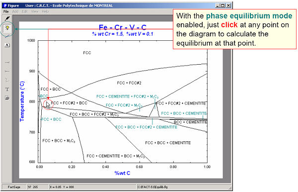
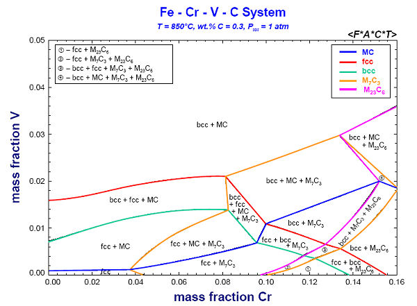
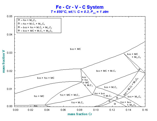
Unlike the Predom module, Phase Diagram can produce predominance area diagrams that also include data from the solution databases. Fig. 4 shows the log10(Po2) vs Cr/(Cr+Fe) phase diagram at 1573 K where the system components are Fe, Cr and O2. The possible phases are the gas and various real solutions taken from the FACT (oxides) and SGTE (alloys) databases. Fig. 5 is the input/output for an isopleth of T(C) vs TiO2/(FeO+TiO2) ratio at 50 mol % Fe in the FeO-TiO2-Fe system again using both FACT and SGTE solution databases. An example of the interactive power of Phase Diagram is the equilibrium calculation shown in Fig. 6 where the user has first selected the phase equilibrium mode and then pointed and clicked at the coordinates 1450ºC and TiO2/(FeO+TiO2) = 0.7. Note, these results would be identical to a calculation with the Equilib module at 1450ºC and 1 atm where the reactants are 0.7 TiO2 + 0.3 FeO + excess Fe.

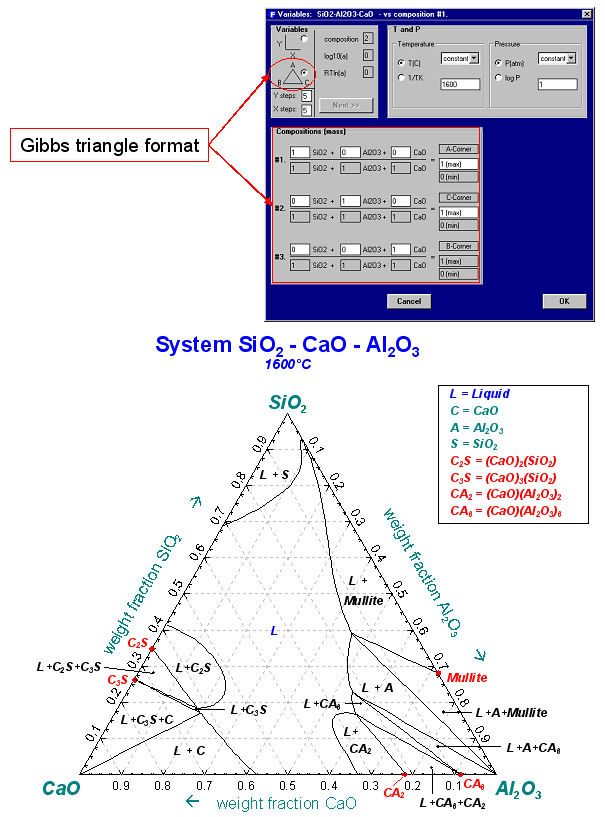
Fig. 7 – CaO-Al2O3-SiO2 system. Top: selection of the Gibbs triangle format, axes and temperature. Bottom: resulting CaO-Al2O3-SiO2 ternary phase diagram at 1600°C (the labels have been edited).

Fig. 7 is the input/output for a Gibbs ternary section of the CaO–Al2O3–SiO2 system at 1600ºC using FACT data.

The calculated diagrams can be stored as figure (*.fig) files, edited by the Figure module, and exported as *.bmp, *.emf and *.wmf files. Examples of the combined use of the Phase Diagram, Equilib and Figure modules to generate phase diagrams are shown in figures 8 to 14.

Fig. 8 – Fe-Cr binary phase diagram: graphical output.

Fig. 9 – Fe-C-W system at 5 wt% W: graphical output.

Fig. 10 – Fe-Cr-V-C system: graphical output.

Fig. 11 – Zero Phase Fraction (ZPF) Lines.

Fig. 12 – FactSage Fe-Cr-V-C system. Mass fraction V versus mass fraction W isopleth at 0.3 wt.% C and 850°C calculated from SGTE data by Phase Diagram and editing the output in the Figure Module.

Fig. 13 – FactSage NaF-NaCl-CaF2-CaCl2 reciprocal system. The liquidus projection was calculated from FACT data by editing the results and ouputs from the Equilib, Phase Diagram and Figure modules.

Fig. 14 – NaCl-KCl-MgCl2 ternary system. The liquidus projection was calculated from FACT data by editing the results and outputs and from Equilib, Phase Diagram and Figure modules.

9. Calphad Optimizer

Click on Download Calphad Optimizer Slide Show (pdf – 93 pages) for detailed information on Calphad Optimizer.

Calphad Optimizer (formerly: OptiSage) is used for the assessment of Gibbs energy data. Various types of experimental data (phase diagram and thermodynamic data, such as enthalpy, activity etc.) can be utilized in order to generate consistent parameters for the Gibbs energies of solutions and compounds that reproduce the experimental input.

Calphad Optimizer has replaced OptiSage in FactSage 8.2. OptiSage is, however, still part of FactSage 8.3 to enable users to access their OptiSage files.

10. Results

Click on Download Results Slide Show (pdf presentation – 19 pages) for detailed information on Results .

Results enables one to post-process the output from calculations performed with Equilib (Equi*.res files) and produce a variety of plots from a single set of equilibrium tables.

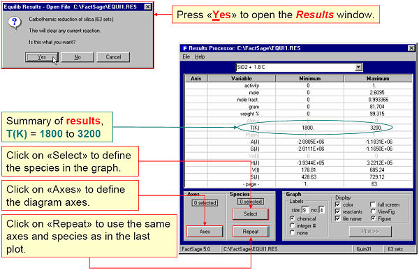
For example, Fig. 1 shows the Results Window accessing Equilib calculations for the carbothermic reduction of silica, C + SiO2, in the temperature range 1800 to 3200 K.

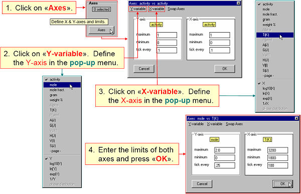
Fig. 2. shows the axes being defined in the Axis Window.

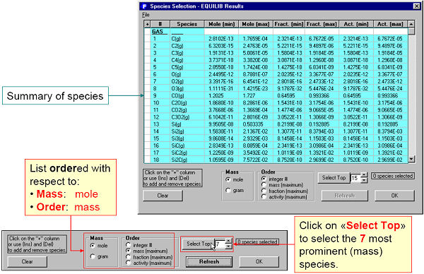
Fig. 3 shows species being selected in the Species Window.

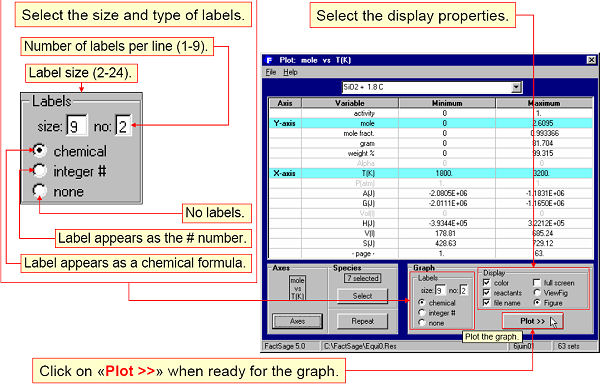
Fig. 4 – Specifying the Graphical Output

Fig. 4 shows the graphical output being specified. The plotted diagram is shown in Fig. 5.

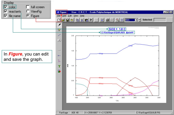
The calculated diagrams can be stored as figure (*.fig) files, edited by the Figure app, and exported as *.bmp, *.emf and *.wmf files.

11. Mixture

Click on Download Mixture Slide Show (pdf presentation – 17 pages) for detailed information on Mixture.

Use Mixture to edit mixtures and streams for input to Equilib.

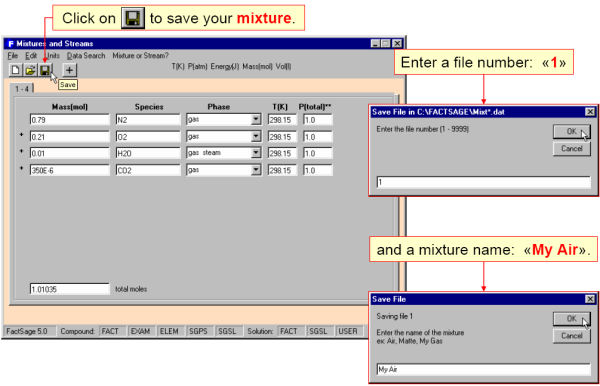
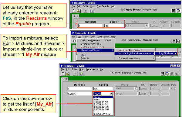
A mixture is a group of compounds that normally would be entered as reactants in the Equilib program. In the Mixture program you can enter these same reactants then store them in a mixture (Mixt*.dat) file. In Equilib you can then import this mixture via the Reactants Window.

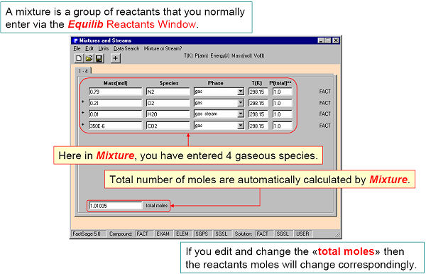
For example, in Fig. 1 four gaseous reactants are defined and in Fig. 2 stored in a mixture file (Mixt1.dat) named ‘My Air’. In Fig. 3 this mixture is imported into Equilib as a reactant.

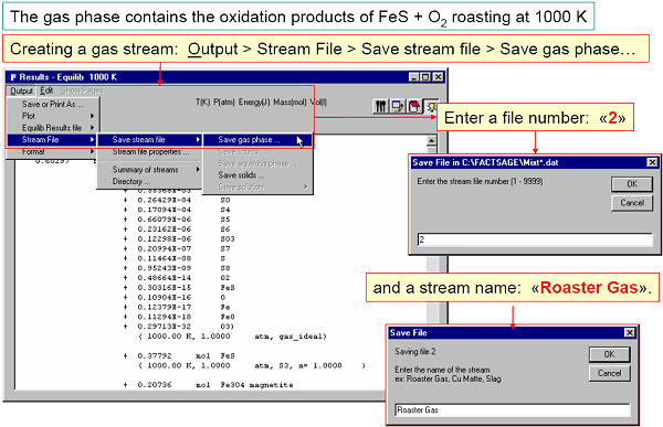
Fig. 3 – Importing “My Air” into Equilib as a single-line mixture

A stream is a list of equilibrated species calculated by Equilib and stored via the Equilib Results Window. The stream can then be edited by Mixture and imported into Equilib via the Reactants Window.

For example, Fig. 4 shows an equilibrated roasted gas phase being stored in a stream. In Fig. 5 the stream is then imported into Equilib as a reactant.

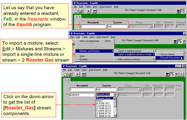
Fig. 5 – Importing “Roaster Gas” into Equilib as a single-line mixture

The mixture or stream can have up to 48 reactants and 32 different elements – for example a complex alloy composition or mineral ore that is repeatedly entered as reactants in Equilib could be easily stored as a single mixture. Note, in Equilib you can import up to 48 different mixtures into a given calculation.

12. Fact-XML

Click on Download Fact-XML Slide Show (pdf presentation – 24 pages) for detailed information on FactXML.

FactXML is an add-in to the Equilib program that enables you to edit the results of a calculation and save customized outputsas templates. There is no limitation to the number of templates.

13. Figure

Click on Download Figure Slide Show (pdf presentation – 47 pages) for detailed information on the Figure.

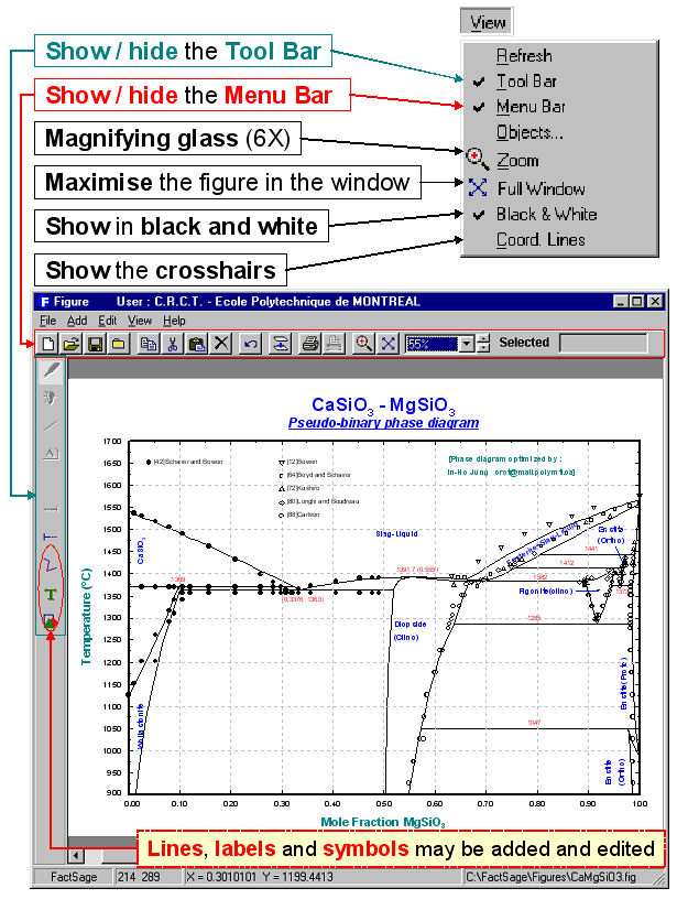
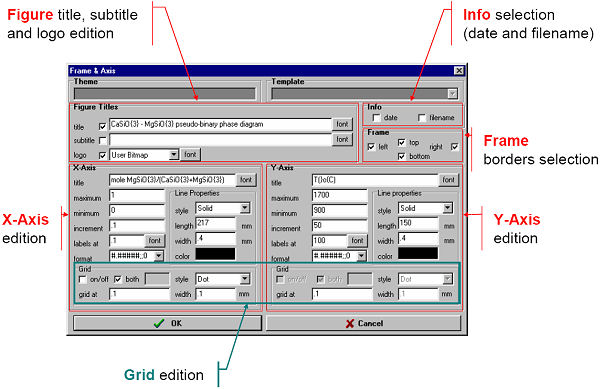
Figure is a generalized plotting program that permits one to display, edit and manipulate the various figures and phase diagrams (*.fig files ) produced by the FactSage programs. It is particularly well suited for treating figures calculated by Phase Diagram. The *.fig files may be opened and edited by Edition, Format, Frame & Axes Windows and Menu Bars.

For example, Figs. 1 and 2 show the use of the View menu bar and the Frame & Axes Window to edit the calculated binary phase diagram for the CaSiO3 – MgSiO3 system.

Fig. 1 – CaSiO3-MgSiO3 system. Example of the View menu bar used to edit calculated phase diagrams.

Figs. 3 to 5 show other edited figures. The resulting diagrams may be exported as *.fig (ASCII for repeated use with Figure), *.bmp, *.emf and *.wmf files (bitmap, enhanced metafile and windows metafile) for subsequent use with other Windows® software.

Fig. 3 – Fe-Cr-V-C system. Mass fraction V versus mass fraction W isopleth at 0.3 wt.% C and 850°C calculated from SGTE data by Phase Diagram and editing the output in the Figure Module.

Fig. 4 – NaF-NaCl-CaF2-CaCl2 reciprocal system. The liquidus projection was calculated from FACT data by editing the results and ouputs from the Equilib, Phase Diagram and Figure modules.

Fig. 5 – aCl-KCl-MgCl2 ternary system. The liquidus projection was calculated from FACT data by editing the results and outputs and from Equilib, Phase Diagram and Figure modules.

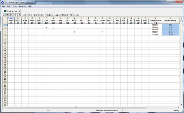
14. Viscosity

A new model for the viscosity of single-phase liquid slags and glasses has been developed. It is distinct from other viscosity models in that it directly relates the viscosity to the structure of the melt, and the structure in turn is calculated from the thermodynamic description of the melt using the Modified Quasichemical Model.

The model requires very few parameters which were optimized to fit the experimental data for pure oxides and selected binary and ternary systems. The viscosities of multicomponent melts and glasses are then predicted by the model within experimental error limits without using any additional parameters.

The model has been checked against the experimental data available for Al2O3-B2O3-CaO-FeO-Fe2O3-K2O-MgO-MnO-Na2O-NiO-PbO-SiO2-TiO2-Ti2O3-ZnO-F melts and for Al2O3-B2O3-CaO-K2O-MgO-Na2O-PbO-SiO2 glasses.

There are two viscosity databases. The database for melts is valid for liquid and supercooled slags with viscosities which are not too high, that is when log10(viscosity, Poise) is less than about 7.5 or ln(viscosity, Pa·S) < 15. In most cases, this corresponds to temperatures above about 900 oC. On the other hand, the database for glasses can be used at and below the glass transition temperatures. In principle, this database is valid over the whole temperature range from liquid melts to glasses, but sometimes it may be slightly less accurate for liquid slags than the first database. Click “Options” to select one of these databases.

Viscosity works for all users who have access to the FToxid database. It is easy to use: select either the Melts or Glass database, select units for the composition, temperature and viscosity, enter a composition (in moles or grams) and a temperature and click the “Calculate” button. A range of compositions and temperatures can be pasted from Excel and the results can be saved in an Excel or text file.

References

1. S. A. Decterov, A. N. Grundy, I.-H. Jung and A. D. Pelton, “Modeling the Viscosity of Aluminosilicate Melts”, In: Computation in Modern Science and Engineering, (Proc. Int. Conf. on Computational Methods in Sciences and Engineering), AIP (American Institute of Physics) Conference Proceedings, Vol. 963, Issue 2, Pt B, Eds. T. E. Simos and G. Maroulis, pp. 404-407 (2007).

2. Grundy A.N., H.-C. Liu, I.-H. Jung, S.A. Decterov and A.D. Pelton, “A Model to Calculate the Viscosity of Silicate Melts. Part I.: Viscosity of Binary SiO2-MeOx Systems (Me = Na, K, Ca, Mg, Al)”. Int. J. Mat. Res., 2008,vol. 99(11), pp. 1185-1194.

3. Grundy A.N., I.-H. Jung, A.D. Pelton and S.A. Decterov, “A Model to Calculate the Viscosity of Silicate Melts. Part II.: Viscosity of the Multicomponent NaO0.5-MgO-CaO-AlO1.5-SiO2 System”. Int. J. Mat. Res., 2008, vol. 99(11), pp. 1195-1209.

4. Kim W.-Y., A.D. Pelton and S.A. Decterov, “A Model to Calculate the Viscosity of Silicate Melts. Part III: Modification of the model for melts containing alkali metals”. Int. J. Mat. Res., 2010, submitted.

5. Brosh E., A.D. Pelton and S.A. Decterov, “A Model to Calculate the Viscosity of Silicate Melts. Part IV: Borosilicate melts”. Int. J. Mat. Res., 2010, submitted.

6. Brosh E., A.D. Pelton and S.A. Decterov, “A Model to Calculate the Viscosity of Silicate Melts. Part V: Borosilicate melts containing alkali oxides”. Int. J. Mat. Res., 2010, submitted.

7. S. A. Decterov, A. N. Grundy and A. D. Pelton, “A Model and Database for the Viscosity of Molten Slags”, Proc. VIII Int’l Conf. on Molten Slags, Fluxes and Salts, Santiago, Chile, pp. 423-431 (2009).

8. Kim W.-Y., A.D. Pelton and S.A. Decterov, “Modeling the Viscosity of Silicate Melts Containing Lead Oxide”. Metall. Mater. Trans., 2010, submitted.